20 Jan, 2026
Auteur: Rik Biel en Matthijs Coster

Programma's bij Numerieke nulpunten

biseCtie_getallen.py

# BISECTIEMETHODE
# uitvoer in getallen

import numpy as np

# >>> Voer hier de functie f(x) in:
def f(x):
    y = x*x*x - 3*x + 1
    return y
# <<<

# >>> Voer hier de startpunten x0 en x1 in:
x0 = 0
x1 = 1.5
# <<<

y0 = f(x0)
y1 = f(x1)
print('startpunten: (x0,y0) = (',x0,',',y0,'), (x1,y1) = (',x1,',',y1,')')

print('iteratie, x2, y2:')
# >>> Voer hier het aantal iteraties in:
for i in range(100):
# <<<
# De volgende benadering x2 ligt midden tussen x0 en x1:
    x2 = (x0 + x1)/2
    y2 = f(x2)
    print(i+1,x2,y2)
# Als y2 = 0, dan is x2 het nulpunt:
    if y2 == 0:
        break
# Anders wordt x0 of x1 aangepast:
    if np.sign(y0) == np.sign(y2):
        x0 = x2
        y0 = y2
    else:
        x1 = x2

biseCtie_grafiek.py

Download bisectie_grafiek.py

# BISECTIEMETHODE
# uitvoer in grafiek

import matplotlib
import matplotlib.pyplot as plt
import numpy as np
import math


# Het plotten van de grafiek van de functie f(x):

matplotlib.use('TkAgg')

# >>> Voer hier het domein [X0,X1] van de grafiek in:
X0 = -2
X1 = 2
# <<<

PN = 601
x = np.linspace(X0,X1,PN)

# >>> Voer hier de functie f(x) in:
Titel = 'f(x) = x^3 - 3x + 1'
f1 = x*x*x - 3*x + 1
# <<<

Xas = 0
Yas = 0
fig = plt.figure(figsize=(6,6),dpi=150)
ax = fig.add_subplot(1,1,1)
ax.spines['left'].set_position(('data',Yas))
ax.spines['bottom'].set_position(('data',Xas))
ax.spines['right'].set_color('none')
ax.spines['top'].set_color('none')
ax.xaxis.set_ticks_position('bottom')
ax.yaxis.set_ticks_position('left')
ax.set_title(Titel)
plt.plot(x,f1,color='r',linewidth=1)
plt.axis('equal')

# >>> Voer hier nogmaals de functie f(x) in:
def f(x):
    y = x*x*x - 3*x + 1
    return y
# <<<

# >>> Voer hier de startpunten x0 en x1 in:
x0 = 0
x1 = 1.5
# <<<

y0 = f(x0)
y1 = f(x1)

# Het plotten van de startpunten:
plt.plot(x0,0,marker='o',markersize=3,color='g')
plt.plot(x0,y0,marker='o',markersize=3,color='r')
plt.plot(x1,0,marker='o',markersize=3,color='g')
plt.plot(x1,y1,marker='o',markersize=3,color='r')

# >>> Voer hier het aantal iteraties in:
for i in range(10):
# <<<
# De volgende benadering x2 ligt midden tussen x0 en x1:
    x2 = (x0 + x1)/2
    y2 = f(x2)
    plt.plot(x2,y2,marker='o',markersize=3,color='r')
    plt.plot(x2,0,marker='o',markersize=3,color='g')
# Als y2 = 0, dan is x2 het nulpunt:
    if y2 == 0:
        break
# Anders wordt x0 of x1 aangepast:
    if np.sign(y0) == np.sign(y2):
        x0 = x2
        y0 = y2
    else:
        x1 = x2

# >>> Kies hier de uitvoer-modus:
# Uitvoer op het scherm:
plt.show()
# Uitvoer in een png-bestand:
# plt.savefig('bisectie.png')
# <<<

regfals_getallen.py

Download regfals_getallen.py

# REGULA FALSI METHODE
# uitvoer in getallen

import numpy as np

# >>> Voer hier de functie f(x) in:
def f(x):
    y = x*x*x - 3*x + 1
    return y
# <<<

# >>> Voer hier de startpunten x0 en x1 in:
x0 = 0
x1 = 1.5
# <<<

y0 = f(x0)
y1 = f(x1)
print('startpunten: (x0,y0) = (',x0,',',y0,'), (x1,y1) = (',x1,',',y1,')')

print('iteratie, x2, y2:')
# >>> Voer hier het aantal iteraties in:
for i in range(100):
# <<<
# De volgende benadering x2:
    x2 = (x0*y1 - x1*y0)/(y1 - y0)
    y2 = f(x2)
    print(i+1,x2,y2)
# Als y2 = 0, dan is x2 het nulpunt:
    if y2 == 0:
        break
# Anders wordt x0 of x1 aangepast:
    if np.sign(y0) == np.sign(y2):
        x0 = x2
        y0 = y2
    else:
        x1 = x2
        y1 = y2

regfals_grafiek.py

Download regfals_grafiek.py

# REGULA FALSI METHODE
# uitvoer in grafiek

import matplotlib
import matplotlib.pyplot as plt
import numpy as np
import math

# Het plotten van de grafiek van de functie f(x):

matplotlib.use('TkAgg')

# >>> Voer hier het domein [X0,X1] van de grafiek in:
X0 = -2
X1 = 2
# <<<

PN = 601
x = np.linspace(X0,X1,PN)

# >>> Voer hier de functie f(x) in:
Titel = 'f(x) = x^3 - 3x + 1'
f1 = x*x*x - 3*x + 1
# <<<

Xas = 0
Yas = 0
fig = plt.figure(figsize=(6,6),dpi=150)
ax = fig.add_subplot(1,1,1)
ax.spines['left'].set_position(('data',Yas))
ax.spines['bottom'].set_position(('data',Xas))
ax.spines['right'].set_color('none')
ax.spines['top'].set_color('none')
ax.xaxis.set_ticks_position('bottom')
ax.yaxis.set_ticks_position('left')
ax.set_title(Titel)
plt.plot(x,f1,color='r',linewidth=1)
plt.axis('equal')


# >>> Voer hier nogmaals de functie f(x) in:
def f(x):
    y = x*x*x - 3*x + 1
    return y
# <<<

# >>> Voer hier de startpunten x0 en x1 in:
x0 = 0
x1 = 1.5
# <<<

y0 = f(x0)
y1 = f(x1)

# Het plotten van de startpunten:
plt.plot(x0,0,marker='o',markersize=3,color='g')
plt.plot(x0,y0,marker='o',markersize=3,color='r')
plt.plot(x1,0,marker='o',markersize=3,color='g')
plt.plot(x1,y1,marker='o',markersize=3,color='r')

# >>> Voer hier het aantal iteraties in:
for i in range(10):
# <<<
# De volgende benadering x2:
    x2 = (x0*y1 - x1*y0)/(y1 - y0)
    y2 = f(x2)
    plt.plot(x2,y2,marker='o',markersize=3,color='r')
    plt.plot(x2,0,marker='o',markersize=3,color='g')
# Als y2 = 0, dan is x2 het nulpunt:
    if y2 == 0:
        break
# Anders wordt x0 of x1 aangepast:
    if np.sign(y0) == np.sign(y2):
        x0 = x2
        y0 = y2
    else:
        x1 = x2
        y1 = y2

# >>> Kies hier de uitvoer-modus:
# Uitvoer op het scherm:
plt.show()
# Uitvoer in een png-bestand:
# plt.savefig('regulafalsi.png')
# <<<

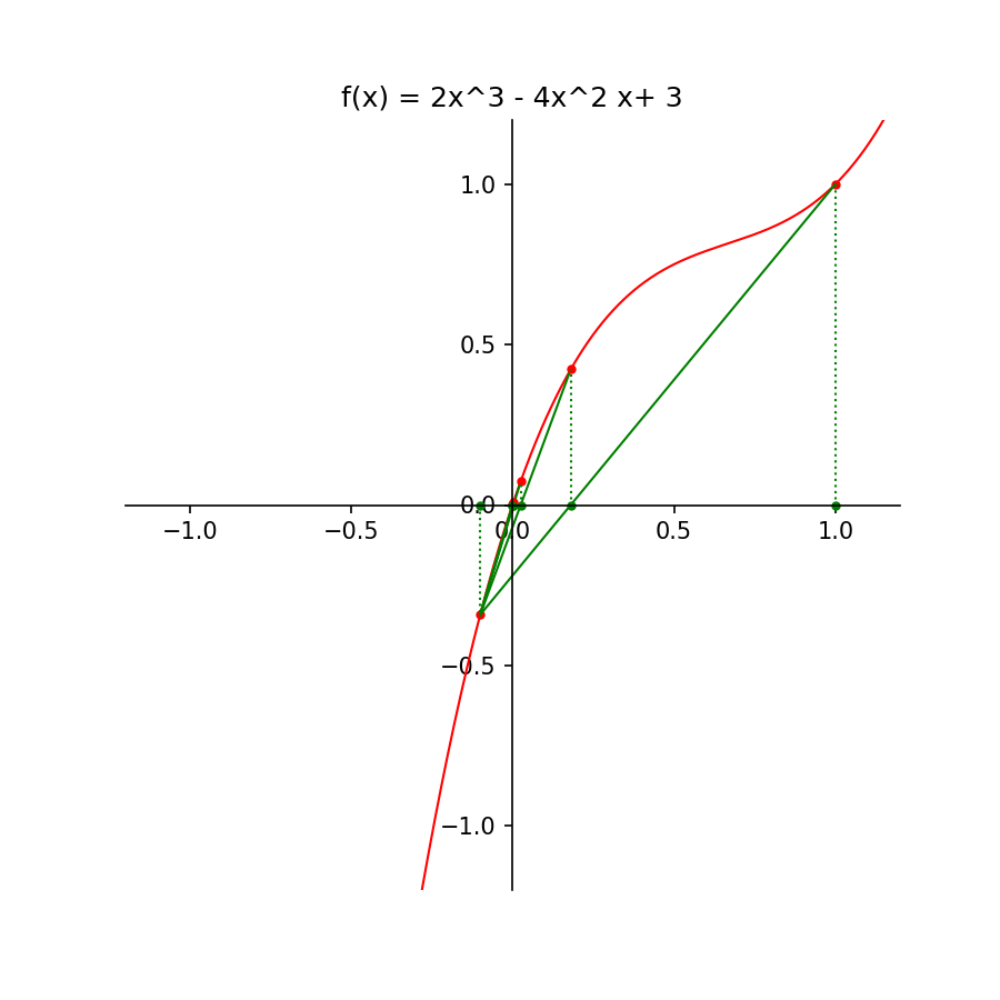
Opgave 3i

Download opgave3i.py

# REGULA FALSI METHODE
# uitvoer in grafiek

import matplotlib
import matplotlib.pyplot as plt
import numpy as np
import math

# Het plotten van de grafiek van de functie f(x):

matplotlib.use('TkAgg')
X0 = -1.2
X1 = 1.2
PN = 601
x = np.linspace(X0,X1,PN)

# De functie f(x) = 2x^3 - 4x^2 + 3x:
Titel = 'f(x) = 2x^3 - 4x^2 x+ 3'
f1 = 2*x*x*x - 4*x*x + 3*x

Xas = 0
Yas = 0
fig = plt.figure(figsize=(6,6),dpi=150)
ax = fig.add_subplot(1,1,1)
ax.spines['left'].set_position(('data',Yas))
ax.spines['bottom'].set_position(('data',Xas))
ax.spines['right'].set_color('none')
ax.spines['top'].set_color('none')
ax.xaxis.set_ticks_position('bottom')
ax.yaxis.set_ticks_position('left')
ax.set_title(Titel)
plt.plot(x,f1,color='r',linewidth=1)
# plt.axis('equal')
ax.set_xlim(-1.2,1.2)
ax.set_ylim(-1.2,1.2)

# De functie f(x) = 2x^3 - 4x^2 + 3x:
def f(x):
    y = 2*x*x*x - 4*x*x + 3*x
    return y

# De startpunten x0 en x1:
x0 = -1
x1 = 1

y0 = f(x0)
y1 = f(x1)

# Het plotten van de startpunten:
plt.plot(x0,0,marker='o',markersize=3,color='g')
plt.plot(x0,y0,marker='o',markersize=3,color='r')
plt.plot([x0,x0],[0,y0],linestyle='dotted',color='g',linewidth=1)
plt.plot(x1,0,marker='o',markersize=3,color='g')
plt.plot(x1,y1,marker='o',markersize=3,color='r')
plt.plot([x1,x1],[0,y1],linestyle='dotted',color='g',linewidth=1)

for i in range(15):
    plt.plot([x0,x1],[y0,y1],color='g',linewidth=1)
    if i > 0:
        plt.plot(x2,y2,marker='o',markersize=3,color='r')
        plt.plot([x2,x2],[0,y2],linestyle='dotted',color='g',linewidth=1)
# De volgende benadering x2:
    x2 = (x0*y1 - x1*y0)/(y1 - y0)
    y2 = f(x2)
    plt.plot(x2,0,marker='o',markersize=3,color='g')
# Als y2 = 0, dan is x2 het nulpunt:
    if y2 == 0:
        break
# Anders wordt x0 of x1 aangepast:
    if np.sign(y0) == np.sign(y2):
        x0 = x2
        y0 = y2
    else:
        x1 = x2
        y1 = y2

# >>> Kies hier de uitvoer-modus:
# Uitvoer op het scherm:
# plt.show()
# Uitvoer in een png-bestand:
plt.savefig('opgave3i.png')
# <<<

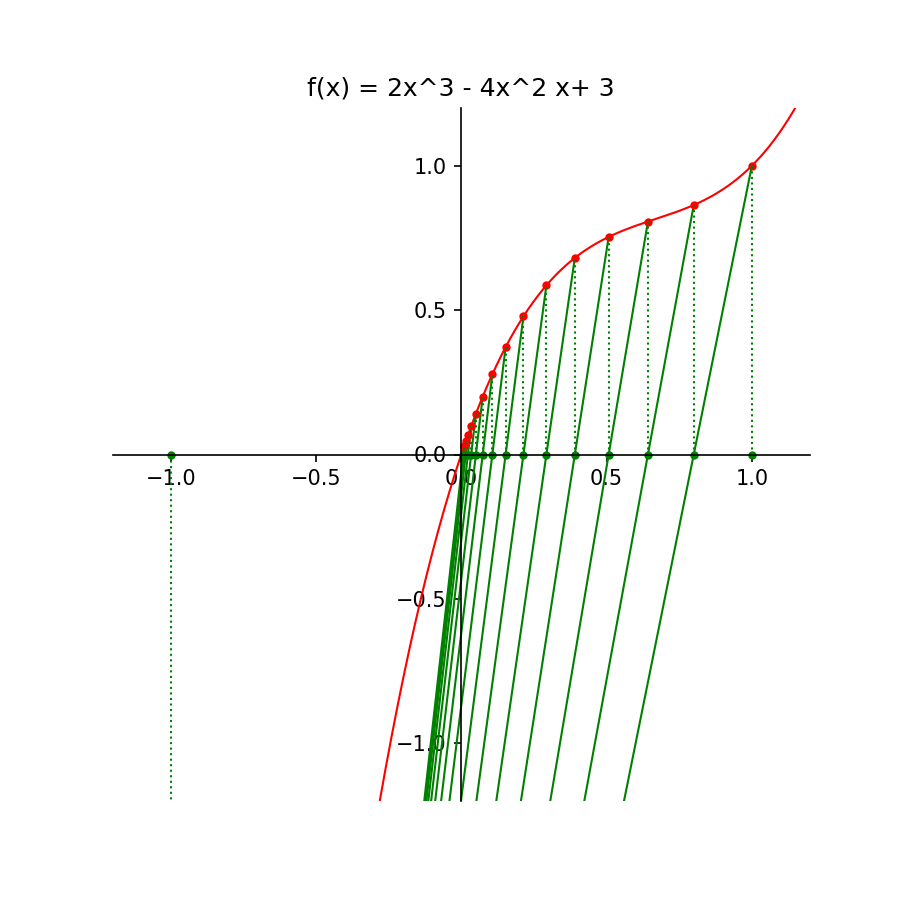
Opgave 3ii

Download opgave3ii.py

# REGULA FALSI METHODE
# uitvoer in grafiek

import matplotlib
import matplotlib.pyplot as plt
import numpy as np
import math

# Het plotten van de grafiek van de functie f(x):

matplotlib.use('TkAgg')
X0 = -1.2
X1 = 1.2
PN = 601
x = np.linspace(X0,X1,PN)

# De functie f(x) = 2x^3 - 4x^2 + 3x:
Titel = 'f(x) = 2x^3 - 4x^2 x+ 3'
f1 = 2*x*x*x - 4*x*x + 3*x

Xas = 0
Yas = 0
fig = plt.figure(figsize=(6,6),dpi=150)
ax = fig.add_subplot(1,1,1)
ax.spines['left'].set_position(('data',Yas))
ax.spines['bottom'].set_position(('data',Xas))
ax.spines['right'].set_color('none')
ax.spines['top'].set_color('none')
ax.xaxis.set_ticks_position('bottom')
ax.yaxis.set_ticks_position('left')
ax.set_title(Titel)
plt.plot(x,f1,color='r',linewidth=1)
# plt.axis('equal')
ax.set_xlim(-1.2,1.2)
ax.set_ylim(-1.2,1.2)

# De functie f(x) = 2x^3 - 4x^2 + 3x:
def f(x):
    y = 2*x*x*x - 4*x*x + 3*x
    return y

# De startpunten x0 en x1:
x0 = -0.1
x1 = 1

y0 = f(x0)
y1 = f(x1)

# Het plotten van de startpunten:
plt.plot(x0,0,marker='o',markersize=3,color='g')
plt.plot(x0,y0,marker='o',markersize=3,color='r')
plt.plot([x0,x0],[0,y0],linestyle='dotted',color='g',linewidth=1)
plt.plot(x1,0,marker='o',markersize=3,color='g')
plt.plot(x1,y1,marker='o',markersize=3,color='r')
plt.plot([x1,x1],[0,y1],linestyle='dotted',color='g',linewidth=1)

for i in range(5):
    plt.plot([x0,x1],[y0,y1],color='g',linewidth=1)
    if i > 0:
        plt.plot(x2,y2,marker='o',markersize=3,color='r')
        plt.plot([x2,x2],[0,y2],linestyle='dotted',color='g',linewidth=1)
# De volgende benadering x2:
    x2 = (x0*y1 - x1*y0)/(y1 - y0)
    y2 = f(x2)
    plt.plot(x2,0,marker='o',markersize=3,color='g')
# Als y2 = 0, dan is x2 het nulpunt:
    if y2 == 0:
        break
# Anders wordt x0 of x1 aangepast:
    if np.sign(y0) == np.sign(y2):
        x0 = x2
        y0 = y2
    else:
        x1 = x2
        y1 = y2

# >>> Kies hier de uitvoer-modus:
# Uitvoer op het scherm:
# plt.show()
# Uitvoer in een png-bestand:
plt.savefig('opgave3ii.png')
# <<<

Programma's bij Numerieke nulpunten

Programma's bij Numerieke nulpunten

biseCtie_getallen.py

biseCtie_grafiek.py

regfals_getallen.py

regfals_grafiek.py

Opgave 3i

Opgave 3ii

Volg ons op